FlowSOM: to analyze flow or mass cytometry data using a self‐organizing map

Backgroud

FlowSOM(Van Gassen et al., 2015)^[1] is one of the available algorithms for flow cytometry and high-dimensional data analysis.

Flow cytometry is a technique which could detect and measure characteristics of many thousand cells or particles per second. The high‐dimensional flow cytometry data have made it possible to detect protein marker expression, allowing cell populations to be characterized in unprecedented detail. Briefly speacking, the first step is going to be a clustering problem for high-dimensional data and FlowSOM could be a solution.

According to Weber and Robinson(2016)^[2], FlowSOM “had extremely fast runtimes, making this method well‐suited for interactive, exploratory analysis of large, high‐dimensional data sets on a standard laptop or desktop computer.”

Algorithm

FlowSOM analyzes flow or mass cytometry data using a self-Organizing Map (SOM). Using a two-level clustering and star charts, FlowSOM helps to obtain a clear overview of how all markers are behaving on all cells, and to detect subsets that might be missed otherwise.

The algorithm consists of four steps:

• reading the data
• building a Self-Organizing Map
• building a minimal spanning tree
• computing a meta-clustering

Reading the data

It actually refers to the preprocessing step. Instead of processing one fcs file, it was recommended to combine several fcs files from an experiment for training. In this way, the model is built on the whole experiment.

There are a lot of different pre-processing methods, we will take scaling as an example. Once all files are read and bundled together, it could be scaled by:

$$c_{ij} = \frac{c_{ij} - mean(c_{1j},.... c_{nj})}{std(c_{1j},.... c_{nj})}$$

This means each column gets a mean value of 0 and a standard deviation of 1, and ensures that each marker gets the same importance in the further processing of the data. (If expert knowledge indicates that one marker should get a higher importance than another one, specific scaling parameters can be set to reflect this in the further course of the algorithm.)

Self‐Organizing Map

A self-organizing map (SOM) is a specific type of artificial neural network (ANN), used for clustering (Kohonen, 1990)^[3]. It is able to convert complex, nonlinear statistical relationships between high-dimensional data items into simple geometric relationships on a low-dimensional display.

It uses unsupervised learning to produce a low-dimensional (typically two-dimensional), discretized representation of the input space of the training samples, called a map, and is therefore also a method to do dimensionality reduction.

SOM

The figure below illustrates how a SOM is trained. The purple blob is the distribution of the training data. The small white disc is the current training datum drawn from that distribution. At first, the SOM nodes are arbitrarily positioned in the data space. The node (highlighted in yellow) nearest the training datum is selected. It’s moved towards the training datum, as are its neighbors on the grid. After many iterations, the grid tends to approximate the data distribution (right).

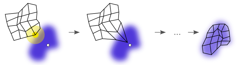Training of a SOM

Training a self-organizing map occurs in several steps:

1. Initialize the weights for each node. The weights are set to small standardized random values.
2. Choose a vector at random from the training set and present to the lattice.
3. Examine every node to calculate which one’s weight is most like the input vector. This will allow you to obtain the Best Matching Unit (BMU). We compute the BMU by iterating over all the nodes and calculating the Euclidean distance between each node’s weight and the current input vector. The node with a weight vector closest to the input vector is marked as the BMU.
4. Calculate the radius of the neighborhood of the BMU. Nodes found within the radius are deemed to be inside the neighborhood of the BMU.
5. Weights of the nodes found in step 4 are adjusted to make them more like the input vector. The weights of the nodes closer to the BMU are adjusted more.
6. Repeat step 2 for N iterations.

Minimum Spanning Tree

The resulting clustering of SOM will be visualized by a minimal spanning tree (MST). MST (Whitney, 1972)^[4] connects the nodes of a graph in such a way that the sum of the weights of the branches is minimal. By doing this, nodes will get connected to the ones they are the most similar to, taking the multidimensional topology of the data in account. Shortly, it is a subset of the edges of a connected, edge-weighted undirected graph that connects all the vertices together, without any cycles and with the minimum possible total edge weight.

Meta Clustering

SOMs can be used to get an immediate clustering, where the number of nodes is set to the expected number of cell types. However, for visualization purposes, it is advantageous to include more nodes than the expected number of clusters. By doing this, cells that are in between cell types can also get a place in the grid and smaller changes in the cell types can be noticed.

The meta-clustering technique conducted on the SOM is hierarchical consensus meta-clustering, which clusters the weights of trained SOM into different groups.

Python Implementation for FlowSOM

The python scripts for FlowSOM is available here.

Reference

[1] Van Gassen, S., Callebaut, B., Van Helden, M.J., Lambrecht, B.N., Demeester, P., Dhaene, T. and Saeys, Y., 2015. FlowSOM: Using self‐organizing maps for visualization and interpretation of cytometry data. Cytometry Part A, 87(7), pp.636-645.

[2] Weber, L.M. and Robinson, M.D., 2016. Comparison of clustering methods for high‐dimensional single‐cell flow and mass cytometry data. Cytometry Part A, 89(12), pp.1084-1096.

[3] Kohonen, T., 1990. The self-organizing map. Proceedings of the IEEE, 78(9), pp.1464-1480.

[4] Whitney, V.K.M., 1972. Algorithm 422: minimal spanning tree [H]. Communications of the ACM, 15(4), pp.273-274.